Its 11:00 PM at night and I have grown bored of revising for the upcoming exams. To alleviate my boredom, I think I am going to spend the next 12 hours or so hacking and blogging.

For a long time, I have been wanting to get my hands dirty with training a convolutional neural network on a GPU instance to recognise breast cell clusters and classify them to be benign or malignant. With the forthcoming days seeming to be terribly occupied with all sorts of revision frenzy, this seems the best time to dive in and see how far I can get with it. Before I dive into the code and setup, I must point out that this is my first attempt at setting up a neural network. A lot of what I will write here would be what I learn as I go along. I am not going to delve into the theoretical details and the math behind making convolutional neural nets work in this blog, I’d like to keep my focus narrowed on the implementation details.

Without further ado, lets get started.

23:34 – Got an Amazon EC2 GPU instance running. I tried installing the CS231N AMI, but I didn’t have GPU instance permissions there, so I reverted to the Oregon region and used the ami-dfb13ebf AMI for having pre installed deep learning frameworks like Tensorflow, Torch, Caffe, Theano, Keras, CNTK amongst others. As I write this, I am also installing Anaconda on the instance so I can put all of my code in a Jupyter notebook and access that remotely from my laptop. I found this guide quite useful on getting the Jupyter notebook up and running on a remote instance – https://chrisalbon.com/jupyter/run_project_jupyter_on_amazon_ec2.html

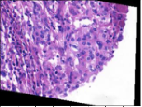
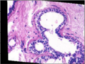
00:27 – GitHub Repository – Check, Packages Installed – Check, Data Transferred to EC2 Instance – Check.  The dataset I’ll be using today consists of ~45 histopathological images. The dataset is available at http://bioimage.ucsb.edu/research/bio-segmentation. Now, 45 images are no where near enough for training and testing a model. That’s why I’ll rely on Keras’ image augmentation features to generate synthetic training data. This would include create images that are flipped, blurred and rotated. To give an example of what the images look like, here are two from the original dataset.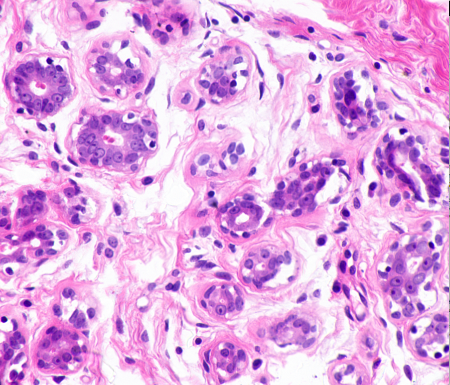

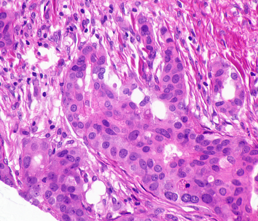
When I first looked at these images, two conflicting feelings engulfed me. On one hand, I found these images quite fascinating; one of the smallest components of our body, undergoing mitosis. On the other hand, it was terrifying, a peek at a disease that is, as Harold Varmus put it, a distorted version of our normal selves.

01:54 – Managed to read the images into my notebook successfully and create the training arrays. Seems like all those all nighters at hackathons have made it easier for me to work well into the night without feeling particularly drowsy. Going to generate about 2500 new images per class.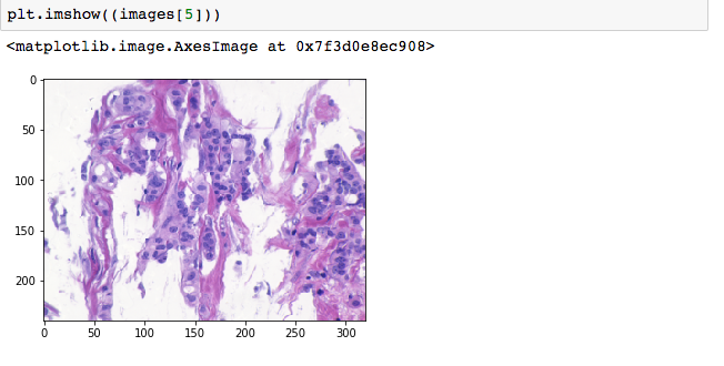

02:08 – Running into errors with generating new images. For some reason, its trying to find JPEG files, whereas my files are TIF. Managed to solve it, the error was arising due to an incorrectly specified path argument for the directory where the images were supposed to be saved. But now, I have a mix of TIF and JPEGs, not sure if that will be alright. Guess I’ll find out. With the augmented image generation done, I now have 5045 images in total. I used an 80:20 split on this.

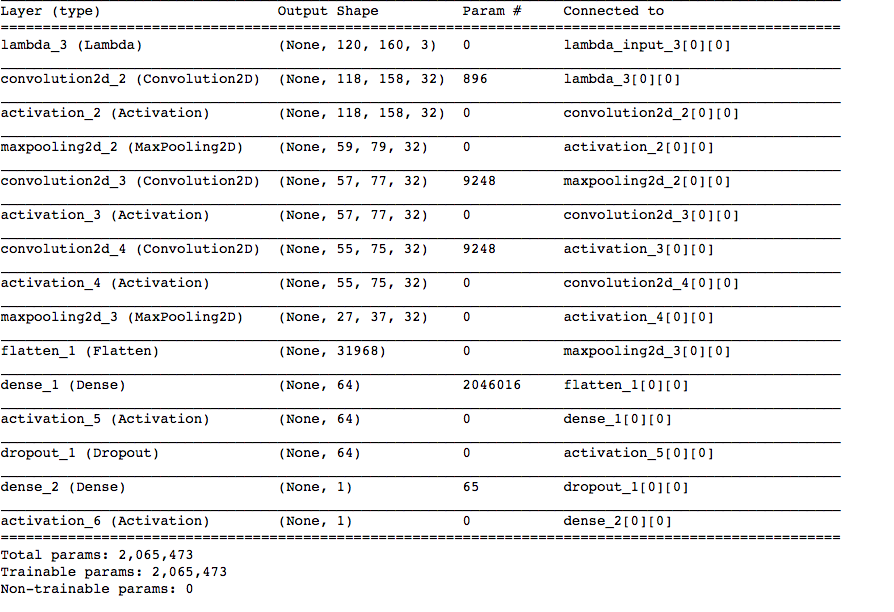
02:50 – Transforming the images and labels was easy. Finally, after 4 hours of data processing, I can finally start training a model. For this, I’ll use an architecture with an input layer followed by convolution, maxpooling, convolution, convolution, max_pooling and fully connected layers. At this point, I’ll also add dropout to prevent over-fitting and then connect it to a fully connected layer that predicts one of the two classes. Will also use the ADAM optimiser and the loss function would be binary_crossentropy. I was predisposed to this architecture because it performed relatively well on the CIFAR-10 database. Enough talk now, time to train it.

03:39 –  The model has started training. The validation accuracy initially was looking quite encouraging, however, it remains to be seen how well it performs on the test set.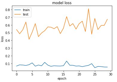

03:46 – 87% accuracy on the test set. Not bad for a baseline model. Still, when I look at the training and validation loss, it seems the model started overfitting. I might have to play around with the parameters/model layers to see if I can make it fit better. However, going to do all that after the exams. This will require a lot of trial and error. Below are some examples that confounded the model.

Here’s an image that was predicted to be benign but is actually malignant.

On the other hand, this one was predicted to be malignant but is actually benign:

The confusion matrix for the model was:

[[415  93]
[ 31 470]]

Giving this confusion matrix was important since the accuracy of the model by itself doesn’t tell us much. A better metric to use is precision and recall. Precision of a model refers to the percentage of true positives guessed, which in this case happens to be 93.04% ( Malignant Predicted and Malignant True / All Malignant Predicted). The recall percentage of the model comes out to 81.7%, which implies that the model was successful in finding the images with malignant tumours roughly 82 times out of 100.

Like I said earlier, this was primarily a learning experience for me. Spending the few hours wrangling with these images taught me:

1. About the effectiveness of CNNs in image recognition tasks due to their ability to extract features without explicitly being given any.
2. A few details about evaluating model performance using the training, validation and testing accuracy.
3. How to leverage openCV and Keras to work with image data.
4. Intuitive details about convolution, max pooling and activation functions.

Now I must call it a day on that and get back to revision, after getting some shut-eye! In the next blog post, I am going to talk about leveraging the Raspberry Pi and a few external components to turn it into a personal assistant device.

Until next time then!

A lot of code was adopted from – https://github.com/dhruvp/wbc-classification/blob/master/notebooks/binary_training.ipynb

Understanding Convolutional Neural Networks – https://medium.com/@ageitgey/machine-learning-is-fun-part-3-deep-learning-and-convolutional-neural-networks-f40359318721

Further reading – Spanhol, Fabio Alexandre, Luiz S. Oliveira, Caroline Petitjean, and Laurent Heutte. “Breast Cancer Histopathological Image Classification Using Convolutional Neural Networks.” 2016 International Joint Conference on Neural Networks (IJCNN) (2016): n. pag. Web.

Code – https://github.com/achadha0111/tumor_classification/blob/master/Cell%20Classification.ipynb